Generating cumulative generating functions
Contents
Generating cumulative generating functions
Generating function string together a sequence of values combined with a formal parameter \(x\) raised to the appropriate power of \(k\). In the case of the probbability generating functions we’re most interested in, these values are coefficients \(\{ p_k \}_{k = 0}^\infty\). It is these coefficients that are the interesting part of the construction.
A probability generating function holds all the information about the distribution and can be manipulated in various ways. To extract the mean degree of nodes, for example, we evaluate
where \(G_0'(x)\) is the first derivative of \(G_0(x)\) which is then executed at 1 to include all the terms. Similar operations can be performed to extract other moments and statistical features. The important point is that these operations are defined purely in terms of the generating function and so work for any such function, not simply one defined by explicit terms. A network with a particular degree distribution will often have a generating function that is not “spelled out” like this, but the operations still work.
(Note that the generating function is a purely formal mathematical device for representing the probability distribution, and the “derivative” is similarly a formal device for manipulating the terms in the formal series: it has nothing whatever to do with rates of change of anything.)
A more complicated feature of a distribution is the cumulative density function or CDF, often written \(P(k \le v)\), capturing the probability of \(k\) being less than or equal to some value \(v\). This is usually defined by integration of the distribution:
where we use a discrete sum since degrees are always whole numbers. Since we have all the information we need encapsulated in the generating function, how can we generate the CDF directly from the probability generating function?
Generating CDFs
Let us re-phrase the problem slightly. Instead of the traditional CDF, what if we are instead interested in the probability of a node having a degree greater or equal to some threshold? – \(P(k \geq v)\). In our case this would then be the probabbility that a node chosen at random had a degree greater than or equal to some value, whcih would be used for example to explore the effects of “hub” nodes with lots of neighbbours. Intuitively is seems that this value is generated by summing the terms of \(p_k\) greater than or equal to \(v\), which are generated by the terms of \(G_0(x)\) in powers of \(x\) greater than or equal to \(v\), discounting all terms in powers of \(x\) less than \(v\).
Having re-phrased the question in this way, it turns out that the answer is known for the general case of generating functions [Wil94].
\(G_0(x)\) is a generating function built from an “ordinary” power series, a sequence of coefficients of the form \(\{ p_k \}_{k = 0}^\infty\). What function generates the sequence \(\{ p_{k + 1} \}_{k = 0}^\infty\)? – in other words, dropping the first term?
which is
Shifting the subscript by one changes the series by a factor determined by the first coefficient. If we want to generate the series from the \(h\)’th term then we use:
So computing \(G_{0, h}(1)\) gives us the probability of a node having a degree greater than or equal to \(h\).
We still need the values of \(p_k\) for \(k \lt h\). We can obtain these in two ways. Firstly, they may be explicitly measurable from an empirical or generated network. If this is the case then by definition we have all the \(p_k\), and so can compute \(P(k \geq h)\) directly as \(P(k \geq h) = \sum_{k \geq h} p_k\).
Secondly, we can obtain \(p_k\) from the \(k\)’th derivative of \(G_0\):
which works for any probbability generating function.
Quick sanity check
Suppose we have a network with \(N = 5\) and the following degree distribution:
\(k\) |
\(p_k\) |
|---|---|
0 |
0 |
1 |
2/5 |
2 |
1/5 |
3 |
2/5 |
What is \(P(k \ge 2)\)? Given the above we can simply read the answer off as \(p_2 + p_3 = 1/5 + 2/5 = 3/5\). The degree sequence is generated by:
Computing the CDF:
\begin{align*} G_{0, 2}(1) &= \frac{G_0(1) - p_0 - p_1 , x }{x^2} \ &= \frac{1 - 0 - 2/5}{1} \ &= 3/5 \end{align*}
Larger sanity check
For a better sanity check, we compare the empirical calculation of \(P(k \geq v)\) for a network against the value generated by the CDF generating function.
import math
import cmath
import functools
import numpy
import networkx
import scipy
import mpmath
import epydemic

import matplotlib
%matplotlib inline
%config InlineBackend.figure_format = 'png'
matplotlib.rcParams['figure.dpi'] = 300
import matplotlib.pyplot as plt
import seaborn
matplotlib.style.use('seaborn')
seaborn.set_context('notebook', font_scale=0.75)
We will start with an ER network of \(N = 10^4\) nodes and \(\langle k \rangle = 8\).
N = int(1e4)
kmean = 8
We create a network with this topology.
g = networkx.fast_gnp_random_graph(N, kmean / N)
Given a network, we can compute the number of nodes of each degree simply by counting.
def nk_g(g):
    degrees = dict()
    for (_, k) in g.degree:
        if k in degrees:
            degrees[k] += 1
        else:
            degrees[k] = 1

    def nk(k):
        if k in degrees:
            return degrees[k]
        else:
            return 0

    return nk
From this we can define a function that gives the empirical value of \(p_k\) for any network.
def pk_g(g):
    nk = nk_g(g)

    def pk(k):
        return nk(k) / g.order()

    return pk
For an ER network, the probability of randomly choosing a node with a given degree is
which we can code directly.
def pk_ER(kmean):
    '''Return a function that computes p_k for a given k on an ER network.'''
    def pk(k):
        return (math.pow(kmean, k) * math.exp(-kmean)) / math.factorial(k)
    return pk
This function, when called with the parameters of the ER network, returns a function for \(p_k\).
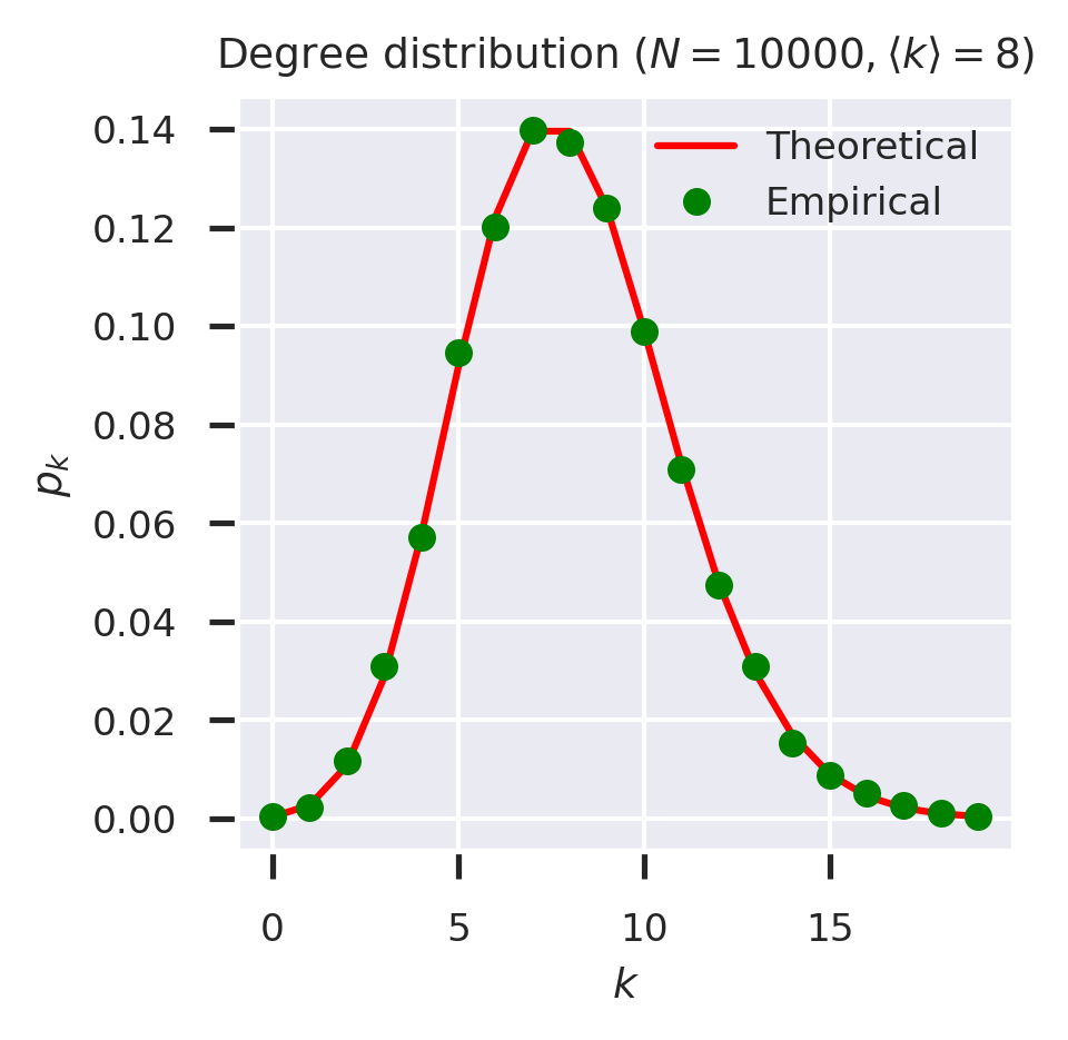
We can check these functions by plotting the theoretical and empirical probabilities on the same axes.
fig = plt.figure(figsize=(3,3))

ks = list(range(20))
theoretical = list(map(pk_ER(kmean), ks))
ds = nk(g)
empirical = [(ds[k] / N if k in ds else 0) for k in ks]

plt.plot(ks, theoretical, 'r-', label='Theoretical')
plt.plot(ks, empirical, 'go', label='Empirical')

plt.xlabel('$k$')
plt.ylabel('$p_k$')
plt.legend(loc='upper right')
plt.title(f'Degree distribution ($N = {N}, \\langle k \\rangle = {kmean}$)')

plt.show()
From the empirical computation of \(p_k\) it is easy to derive \(P(k \geq v)\) by summing -up the probabilities. Again, we define a function that, given a function that computes \(p_k\), returns a function that computes \(P(k \geq v)\)
def cdf_g(g):
    '''Return the CDF of the given network.'''

    def cdf(v):
        ds = nk(g)
        gte = 0
        for k in ds:
            if k >= v:
                gte += ds[k]
        return gte / g.order()

    return cdf
cdf_g(g)(10)
0.2815
Let us now turn to the generating function approach. The degree distribution for an ER network is generated [NSW01] by
def G0_ER(kmean):
    '''Return the degree generating function for an ER network with mean degree kmean.'''

    def G0(x):
        return cmath.exp(kmean * (x - 1))   # note use of complex exponentiation

    return G0
Given a degree generating function we can extract \(p_k\) by taking derivatives. If we know the generating function we can sometimes perform this symbolically, but a numerical solution would work for any generating function, notably for those built piecemeal from arbitrary distributions. The naive approach suffers from numerical instability, but [NSW01] suggests a solution: differentiate the function using the Cauchy contour integral and the residue theorem:
where \(r\) is the radius of a small region around the point of interest.
def differentiate(f, a, n=1, r=1.0, dx=1e-6):
    '''Compute the n'th derivative of f at a using a Cauchy contour integral of radius r.'''

    # make sure the function vectorises
    if not isinstance(f, numpy.vectorize):
        f = numpy.vectorize(f)

    z = r * numpy.exp(2j * numpy.pi * numpy.arange(0, 1, dx))
    return math.factorial(n) * numpy.mean(f(a + z) / z**n)
We can then use this to extract the individual degree probailities by differentiating the degree denerating function the appropriate number of times and evaluating the derivative at zero.
def pk_gen(G0):
    '''Return p_k from the degree generating function G0.'''

    @functools.lru_cache()
    def pk(k):
        return differentiate(G0, 0, dx=1e-2, n=k).real / math.factorial(k)

    return pk
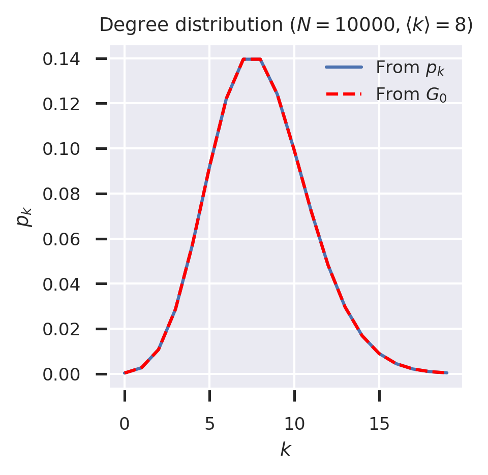
(Since degrees are always real, and indeed integer, it’s safe to extract only the real part of the computed derivative.) We can now see whether the degrees from the degree distribution align with those extracted from the generating function.
fig = plt.figure(figsize=(3, 3))

ks = range(20)
p = pk_ER(kmean)
G0 = G0_ER(kmean)
from_pk = [p(k) for k in ks]
from_G0 = [differentiate(G0, a=0., n=k, r=1., dx=1e-2).real / math.factorial(k) for k in ks]

plt.plot(ks, from_pk, label='From $p_k$')
plt.plot(ks, from_G0,color='r', label='From $G_0$', linestyle='--')
plt.legend()
plt.xlabel('$k$')
plt.ylabel('$p_k$')
plt.legend(loc='upper right')
plt.title(f'Degree distribution ($N = {N}, \\langle k \\rangle = {kmean}$)')
plt.show()
The CDF generating function can then be synthesised from the degree distribution generating function.
def cdf_gen(G0, v):
    '''Return the CDF at v from the degree generating function G0.'''

    @functools.lru_cache()
    def G0_v(x):
        pk = pk_gen(G0)
        s = 1 - sum([pk(k) for k in range(v)])
        return s / math.pow(x, v)

    return G0_v
cdf_gen(G0_ER(kmean), 10)(1)
0.28337574127298937
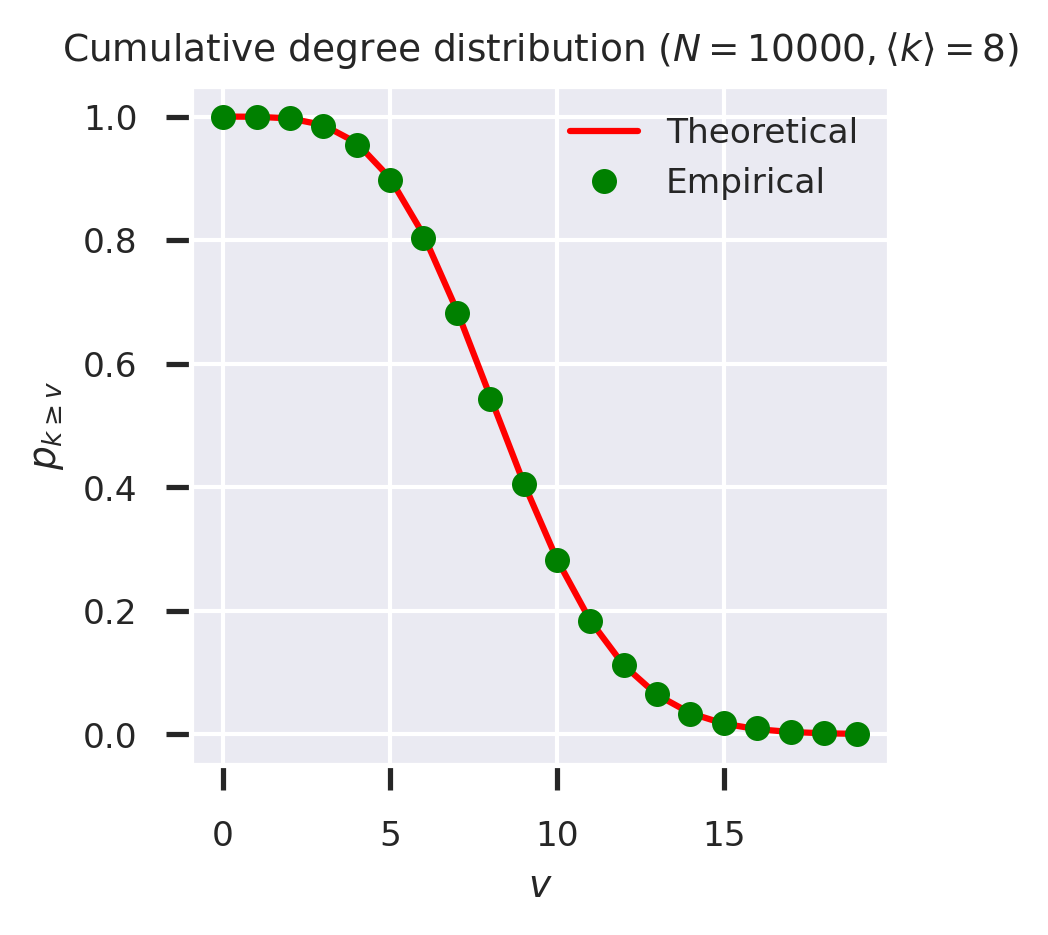
To check the workings of the CDF generating function we can again plot the empirical and theoertical results side by side.
fig = plt.figure(figsize=(3,3))

ks = list(range(20))
theoretical = list(map(lambda k: cdf_gen(G0_ER(kmean), k)(1), ks))
empirical = list(map(cdf_g(g), ks))

plt.plot(ks, theoretical, 'r-', label='Theoretical')
plt.plot(ks, empirical, 'go', label='Empirical')

plt.xlabel('$v$')
plt.ylabel('$p_{k \geq v}$')
plt.ylim([-0.05, 1.05])
plt.legend(loc='upper right')
plt.title(f'Cumulative degree distribution ($N = {N}, \\langle k \\rangle = {kmean}$)')

plt.show()
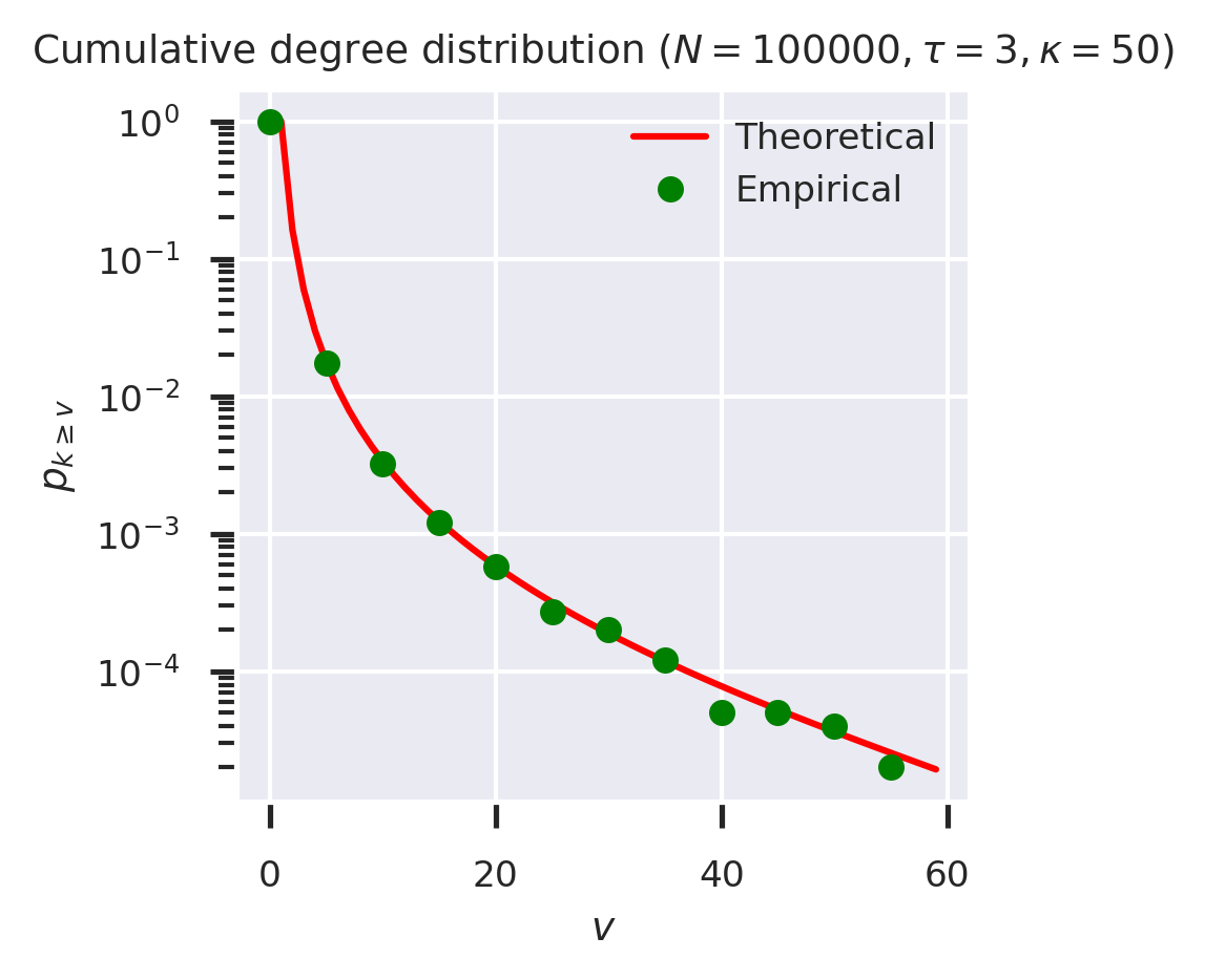
Our claim was that this technique can work with any generating function. To test this, let’s create a powerlaw-with-cutoff degree distribution and apply the same CDF process to its generating function, comparing with the empirical solution.
N_PLC = int(1e5)
tau = 3
kappa = 50
params = dict()
params[epydemic.PLCNetwork.N] = N_PLC
params[epydemic.PLCNetwork.EXPONENT] = tau
params[epydemic.PLCNetwork.CUTOFF] = kappa

g_plc = epydemic.PLCNetwork(params).generate()
The degree distribution is generated [NSW01] by
which again can be coded directly.
def G0_PLC(tau, kappa):
    '''Return the degree generating function for a powerlaw-with-cutoff network with exponent tau and cutoff kappa.'''

    @functools.lru_cache()
    def G0(x):
        return mpmath.polylog(tau, x * math.exp(-1 / kappa)) / mpmath.polylog(tau, math.exp(-1 / kappa))

    return G0
Plotting theoretical and empirical results again, this time on a log-linear scale, gives:
fig = plt.figure(figsize=(3,3))

ks = list(range(60))
theoretical = list(map(lambda k: cdf_gen(G0_PLC(tau, kappa), k)(1), ks))
empirical = list(map(cdf_g(g_plc), ks))

plt.plot(ks, theoretical, 'r-', label='Theoretical')
plt.plot(ks[::5], empirical[::5], 'go', label='Empirical')

plt.xlabel('$v$')
plt.ylabel('$p_{k \geq v}$')
plt.yscale('log')
plt.legend(loc='upper right')
plt.title(f'Cumulative degree distribution ($N = {N_PLC}, \\tau = {tau}, \\kappa = {kappa}$)')

plt.show()