Clearly saving battery power means getting the XBee radio to sleep at the behest of the Arduino. This turns out to be fairly simple, but does require modifying the XBee shield slightly.

Our previous measurements indicate that the XBee draws about 45mA of current — something we have to save for battery-powered nodes. Fortunately XBee radios have a hardware-controlled sleep mode, so the Arduino can sleep the radio when not in use.

Since XBees work as a mesh network, it’s clearly going to be an issue as to when a radio sleeps, and for how long — since when asleep the radio can’t route packets, and so the network starts to break down. But that’s a higher-level concern: for the moment, we’ll focus on the mechanics of getting the XBee to sleep.

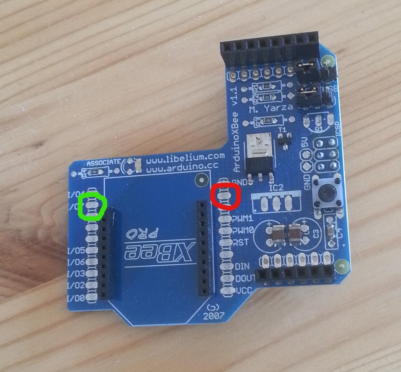
The basic mechanism is simple, and involves hardware and software. At the hardware level, the XBee uses pin 9 (shown in red right) as a control pin. This pin can be used to sleep the radio: setting it to 3,3V (“high” or “asserted”) causes the radio to sleep; setting it to 0V (“low” or “deasserted”) wakes the radio up. The XBee only takes account of the pin when in certain sleep modes, however: these are analogous to the Arduino’s sleep modes. This is the software part: the XBee needs to be placed into the correct sleep mode, and can then be controlled from the Arduino.

Also note I/O line 7, pin 12 (in green): we’ll come back to this later.

We’ll deal with the hardware part first, and then the software.

Getting access to the sleep pin

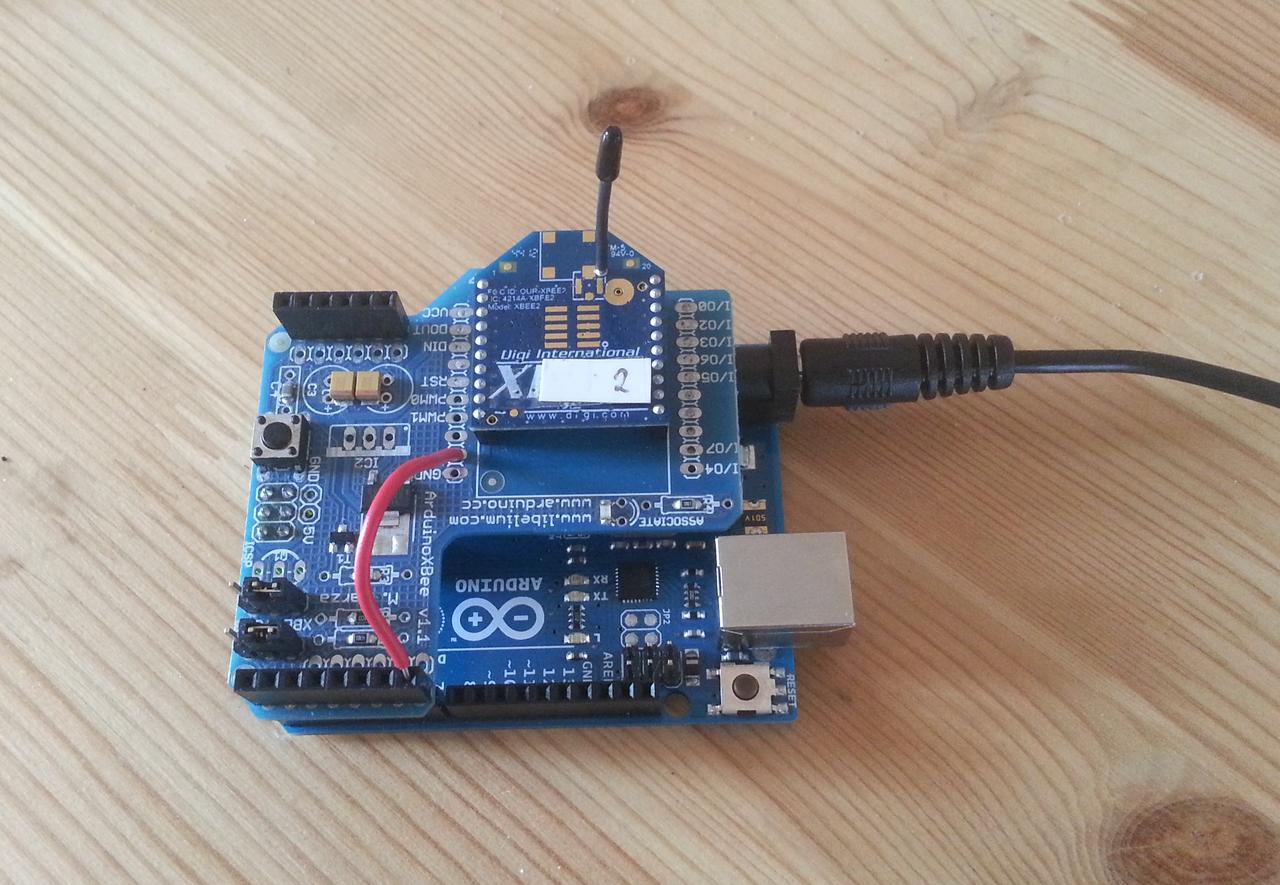
The XBee shield doesn’t connect the sleep pin to anything by default, so to control it we have to connect it. There are several ways we could do this, with the simplest being to solder a wire from the pan on pin 9 to an appropriate header on the shield, which is then connected to a digital pin on the Arduino. For simplicity we’ll start with a wire that’s long enough to reach any header: we’ll actually plug it into the header for the Arduino’s D7 pin.

There’s a slight concern about voltage levels in this approach, as the Arduino operates at 5V while the XBee uses 3.3V. Experimentally this doesn’t seem to make a difference; for a production system we’d probably want to create a resistor network to drop the voltage to that needed by the radio, to avoid any risk of damage. We’d also probably want to solder a header to XBee pin 9’s pad to make it easier to connect the wiring.

Setting the sleep mode

The XBee’s sleep mode is controlled by a single AT command called (unsurprisingly) SM. The default (SM 0) is for the radio to be on all the time; SM 1 selects the pin-sleep mode described above, and is the one we’ll be using as it places the radio under the (hardware) control of the Arduino. (There are other sleep modes where the radio sleeps under the control of its own internal timer. Some projects use the radio’s timer to wake the Arduino rather than the other way round: we prefer to keep the Arduino in control.)

Setting the sleep mode is simply a matter of issuing the appropriate AT command. However, as with a lot of things to do with hardware, we have to set things up slightly first.

The first issue concerns the setting of the XBee’s sleep pin. If we select pin-sleep mode with the pin high, the XBee will sleep immediately, which might not be what we intended. So if we’ve connected the sleep pin to D7, we need to set things up so that the pin is low to keep the radio awake, and then select its sleep mode:

#define XBEE_SLEEP 7                // Xbee sleep pin on D7

void setup() {
   ...
   pinMode(XBEE_SLEEP, OUTPUT);     // sleep control
   digitalWrite(XBEE_SLEEP, LOW);   // deassert to keep radio awake when sleep mode selected
   ...
}

(Some early mistakes showed that — contrary to what might be expected — the sleep pin defaults to high (send radio to sleep) rather than low. So this step is important.)

The next issue concerns the rather intricate behaviour of the XBee’s other pins when sleeping. When the radio enters sleep mode, it asserts its I/O 7 line (pin 12) so that external devices know that it’s asleep. This could be used to make sure that external peripherals wake up only when the radio is active, but for some reason the XBee shield’s designers have connected this pin to the Arduino’s reset line, which means that sleeping the radio will reset (and in fact freeze) the Arduino. Some posts suggest that solving this requires cutting lines on the shield, which might have been true for earlier shields but now isn’t: we simply need to disable the output of this pin, using another AT command:

atCommand("D7", 0);

This disables the XBee’s D7 line (not to be confused with the Arduino’s D7 line, which we’ve attached to the XBee’s sleep pin), which is enough to stop the Arduino freezing. on sleep. (Yes, this did take quite a while to work out, since you ask…)

We can now put all this together to place the XBee into SM 1  and let the Arduino sleep it at will:

#define LED 13
#define XBEE_SLEEP 7                // XBee sleep pin on D7

void setup() {
   pinMode(LED, OUTPUT);            // LED signal
   pinMode(XBEE_SLEEP, OUTPUT);     // sleep control
   Serial.begin(9600);
   radio.setSerial(Serial);

   digitalWrite(XBEE_SLEEP, LOW);   // deassert to keep radio awake when sleep mode selected
   if(atCommand("D7", 1) | atCommand("SM", 1)) {
      // AT commands failed, flash frantically
      ...
   }
   ...
}

Note that we’ve used local AT commands to set the radio’s mode. It’s also possible to do this statically using X-CTU.

Results

The results of all this hacking are that the Arduino can put the XBee into sleep mode whenever it wants to simply by asserting D7. The voltages on pins are maintained even when the Arduino itself sleeps, so it can put the radio to sleep and then sleep itself, wake up and wake up the radio.

Measuring current shows that the sleeping Arduino and XBee draw abour 35mA, the same as an Arduino alone. This makes sense, as the XBee datasheet suggests that when sleeping it draws current in the microamp range — far too small for a normal ammeter to measure, and dwarfed by the quiescent current of the Arduino board (which still needs some work).

Waking the radio happens quickly when the sleep pin is deasserted, but it seems to take some time to re-connect to the mesh co-ordinator: around 7s, in fact, which is a little strange and needs some more exploration.

Controlling the XBee requires issuing AT commands. The XBee library has the low-level machinery to do this.

AT commands are the basis for controlling almost all modems, and the XBee is no different. In API mode, AT commands are issued in a similar manner to sending data. The Arduino XBee library has the low-level code needed, which can be wrapped into a slightly easier-to-use form.

The basic approach is to send an AT command request packet and then read a returned packet acknowledging the command. For the moment we’ll stick to “setting” commands, where the AT command takes an integer parameter: the other are needed less frequently. We construct the request packet, send it, read the response, and check that all went well. This isolates the rest of the program from the message exchange, but also hides the exact nature of any error.

#include <XBee.h>

XBee radio;

int atCommand( char *command, uint8_t param ) {
  // send local AT command
  AtCommandRequest req = AtCommandRequest((uint8_t *) command, (uint8_t *) &amp;param, sizeof(uint8_t));
  radio.send(req);

  // receive response frame
  AtCommandResponse res = AtCommandResponse();
  if(radio.readPacket(500)) {                               // read packet from radio
     if(radio.getResponse().getApiId() == AT_RESPONSE) {    // right type?
       radio.getResponse().getAtCommandResponse(res);
       if(res.isOk()) {                                     // not an error?
         return 0;
       }
     }
  }

  // if we get here, return a failure
  return 1;
}

This function can be used to issue the different control codes for the radio. Some parameters can be set using X-CTU when the radio firmware is installed, but commands are sometimes needed at run-time too.

Some initial measurements of power consumption.

How much power does Arduino sleep mode save? The simplest way to work this out is to power an Arduino from a battery pack and measure the current being drawn in the different modes. A simple program to demonstrate the different modes is:

• Normal delay() loop
• Deep sleep for a period (deep sleep)
• Flash the LED (awake)
• Flash the LED differently while sending out radio messages (awake and transmitting)

The results are as follows:

The good news is that SleepySketch makes it very easy to access the deep sleep mode, and to stay in it by default. This is good, as the normal approach of using delay() is quite power-hungry. The bad news is that the “at rest” power consumption of an Arduino even in deep sleep  — the quiescent current being drawn by the voltage regulator and other components on the board, regardless of what the microcontroller is doing — is about 35mA, with an XBee drawing an additional 40mA.There is very little difference in power whether the radio is transmitting or not (although the current being drawn looked more variable when transmitting, suggesting that there’s some variation happening faster than the ammeter’s sample time).

The radio isn’t put to sleep when the Arduino is asleep, which is clearly something that needs to happen: it draws power even when the Arduino is incapable of using it. Something to explore. Potentially more serious is the power being drawn when the Arduino is asleep. A battery pack with 4 x 1500mAH batteries will be drained in about 7 days (6000mAH / 35mA) even with the system asleep all the time.

[UPDATE 1Aug2013: made the table layout a bit clearer.]

The current focus on “big data” may be obscuring something more interesting: it’s often not the pure size of a dataset that’s important. The idea of extracting insight from large bodies of data promises significant advances in science and commerce. Given a large dataset, “big data” techniques cover a number of possible approaches:

• Look through the data for recurring patterns (data mining)
• Present a summary of the data to highlight features (analytics)
• (Less commonly) Identify automatically from the dataset what’s happening in the real world (situation recognition)

It’s funny how even early experiences change the way you think about a design. Two minor changes to SleepySketch have been suggested by early testing.

The first issue is obvious: milliseconds are a really inconvenient way to think about timing, especially when you’re planning on staying asleep for long periods. A single method in SleepySketch to convert from more programmer-friendly days/hours/minutes/seconds times makes a lot of difference.

The second issue concerns scheduling — or rather regular scheduling. Most sampling and communication tasks occur on predictable schedules, say every five hours. In an actor framework, that means the actor instance (or another one) has to be re-scheduled after the first has run. We can do this within the definition of the actor, for example using the post() action:

class PeriodicActor : public Actor {
   void post();
   void behaviour();
}

...

void PeriodicActor::post() {
   Sleepy.scheduleIn(this, Sleepy.expandTime(0, 5));
}

(This also demonstrates the expandTime() function to re-schedule after 0 days and 5 hours, incidentally.) Simple, but bad design: we can’t re-use PeriodicActor on a different schedule. If we add a variable to keep track of the repeating period, we’d be mixing up “real” behaviour with scheduling; more importantly, we’d have to do that for every actor that wants to run repeatedly.

A better way is to use an actor combinator that takes an actor and a period and creates an actor that runs first re-schedules the actor to run after the given period, and then runs the underlying actor. (We do it this way so that the period isn’t affected by the time the actor actually takes to run.)

Actor *a = new RepeatingActor(new SomeActor(), Sleepy.expandTime(0, 5));
Sleepy.scheduleIn(a, Sleepy.expandTime(0, 5))

The RepeatingActor runs the behaviour of SomeActor every 5 hours, and we initially schedule it to run in 5 hours. We can actually encapsulate all of this by adding a method to SleepySketch itself:

Sleepy.scheduleEvery(new SomeActor(), Sleepy.expandTime(0, 5));

to perform the wrapping and initial scheduling automatically.

Simple sleepy sketches can now be created at set-up, by scheduling repeating actors, and we can define the various actors and re-use them in different scheduling situations without complicating their own code.